Uncertainty and sensitivity functions and implementation

We implemented many scripts and functions to perform uncertainty and sensitivity analysis (for PRCC and eFAST) and display scatter plots (for sample-based methods only). The scripts are written in Matlab©¹ and they are available at the links below. The Statistical Toolbox is required to run them. The ODE model in section 4.2 is used as a template to illustrate the functions.

Tables 1 and 2 lists and describes all the scripts/functions implemented in Matlab for our US analysis. For the details are included at the beginning of each file. Figures 1 and 2 illustrate a diagram of how LHS-PRCC and eFAST is implemented in Matlab.

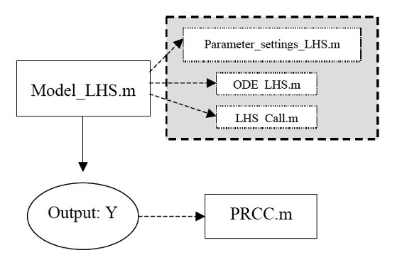
Figure 1: LHS-PRCC diagram. Model_LHS calls the functions in the grey box and produces the output Y. The function PRCC needs the output Y and the LHS matrix (generated by LHS_call) to compute PRC coefficients.

LHS-PRCC

We implemented serveral different functions to perform uncertainty and sensitivity analysis and interpret the results with LHS-PRCC. The LHS-PRCC diagram (Figure 1) describes how the Matlab scripts are connected to each other and how US analysis is performed. We also have three Matlab functions to display scatter plots of LHS values versus output for the sensitivity analysis. They also calculate the correspondent sample-based correlation coefficient (CC_PLOT, RCC_PLOT and PRCC_PLOT, see Table 1 for details).

Table 1: file names and descriptions for LHS-PRCC Matlab scripts and functions. A more detailed description is available in each of the file headers.

The graphical scripts are encoded in the functions CC_PLOT( ), RCC_PLOT( ) and PRCC_PLOT( ). They all have same inputs: LHS matrix (N x k), output matrix (time x N), the time point under study, the type of plot (linear or log scale) for the data and a vector of strings with the labels of the parameters varied in the LHS scheme. Each script returns a number of plots equal to the number of columns of LHS matrix (LHS submatrices can be given as input as well): the title of the plot shows the correlation index (Pearson for CC_PLOT, Spearman for RCC_PLOT and PRCC for PRCC_PLOT) with the respective p-value.

PRCC_PLOT is particularly useful because plots the transformed data for calculating PRCC (residuals of the partial regression of LHS matrix and the output, see PRCC section). If nonlinearities and no clear monotonicities are displayed by these plots, then a variance-based method is recommended in order to compare and confirm US analysis results.

Our PRCC function (PRCC.m) calculates PRCCs and their significances. The output is a matrix of PRCCs (s x k) with 3 possible different p-value matrices (s x k) for significance of the PRCCs: standard, Bonferroni correction and Benjamini and Hochberg False Discovery Rate correction (see Supplement B). Our implementation does not allow for singular LHS matrix. If 2 or more columns (rows) are linearly correlated, the function returns NaN. To eliminate the problem and check for correlation between inputs, Matlab©¹ function corr can be run on the LHS matrix and eventually choose only one of the inputs that are perfectly correlated (discarding the columns of the others) before running PRCC again.

Table 2: file names and descriptions for eFAST Matlab scripts and functions.

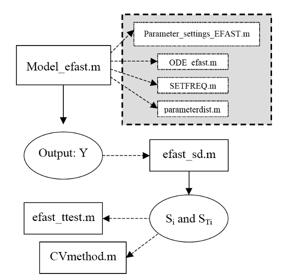
Our eFAST script is a little more sophisticated because the sampling and the sensitivity index generation is embedded with the model output generation. See Table 2 for details on all the scripts and functions described in Figure 2.

Figure 2: EFAST diagram. Model_efast calls the function in the grey box and produces the output Y. The function efast_sd needs the output Y to generate first and total-order coefficients S_i and S_Ti. Efast_ttest tests for indexes that are significantly different from the dummy and the CVmethod check for the reliability of the t-test results.